Fourier

This project was to perform a Discrete Fourier Transform (DFT) on a sampled signal and determine its power spectrum. Each example produces a signal determined by an equation f(t). The first graph displays the original source signal. The second graph shows the discrete data points used in the DFT. The third graph charts the magnitude of each frequency and its phase angle in pi radians. The final graph plots the reconstructed signal using its power spectrum. The charting control is an example of one of the controls developed for Mapromar.

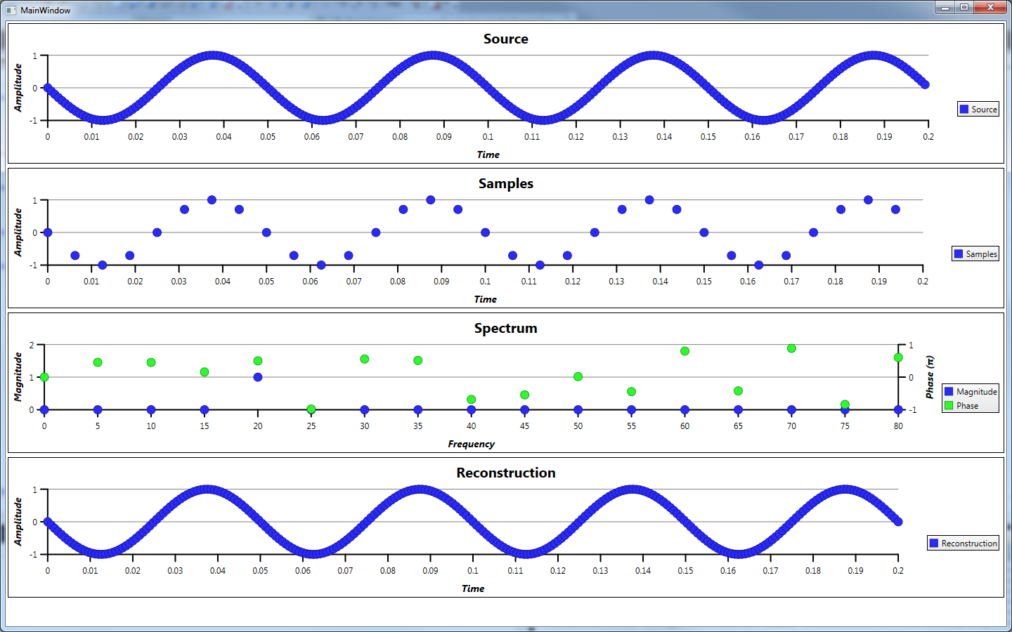
Example 1

Example 1 is a simple cosine wave at 20Hz with a phase shift of 0.5π radians. The spectrum analysis clearly shows only one frequency at 20Hz with its phase angle.

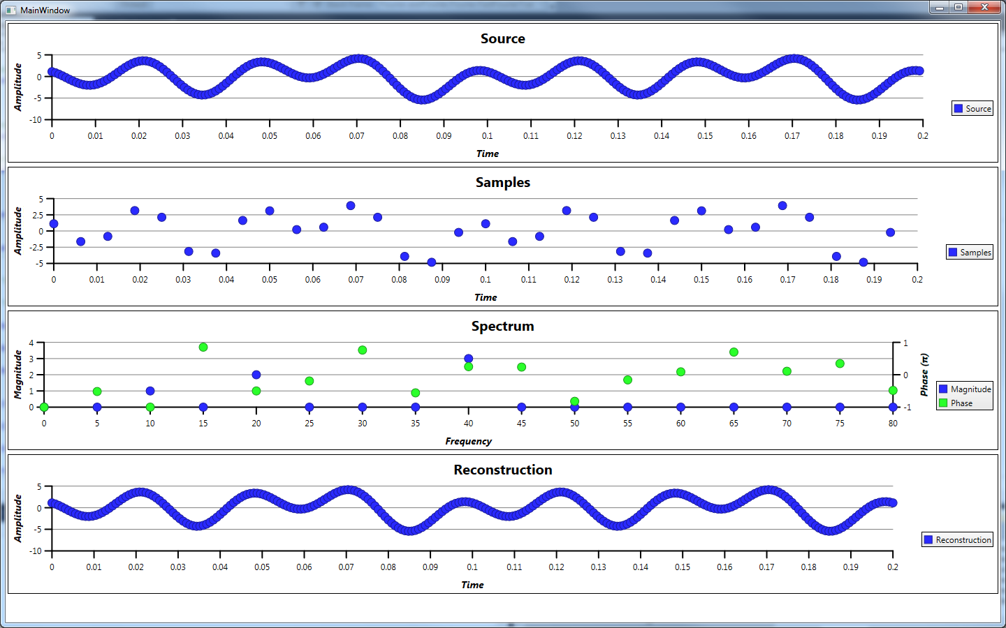
Example 2

Example 2 is a summation of cosine waves at 10Hz, 20Hz and 40Hz with a magnitude of 1, 2, 3 and a phase shift of -π, -0.5π and 0.25π radians respectively. The spectrum analysis shows these frequencies and its phase angle.

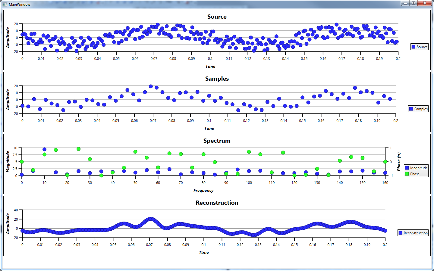
Example 3

Example 3 is a simple cosine wave at 10Hz with a magnitude of 10 and a phase shift of 0.5π radians. Random noise with a magnitude of ±10 is also added to disturb the signal. Despite the noise being added, the spectrum analysis still shows a large magnitude at a frequency of 10Hz with its phase angle. However, the reconstructed signal does not resemble the original closely.

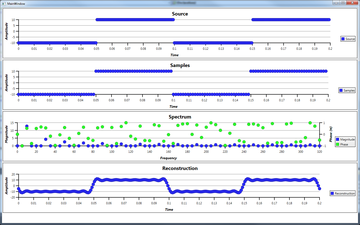
Example 4

Example 4 is a square wave with a magnitude of ±10. Square waves are the result of summing up many different frequencies which can be seen in the spectrum analysis.